Mamba explained and implemented
The Mamba SSM architecture, explained and implemented in Pytorch
Hello everyone, today I will be going through a Mamba implementation written in PyTorch. I will be basing it off this excellent Github repository on a simple but still relatively performant implementation of Mamba. Note we will not cover any of the hardware-aware optimizations.
What is Mamba
So first, introduction, what is Mamba? Mamba is basically SSM made good, introduced in this paper. Then what is SSM? Simply put,
\[\displaylines{ \dot{x} = Ax + Bu\\ y = Cx + Du }\]Where $x$ is the hidden state, $u$ represents the input at a timestep, and $y$ represents the output of the state space machine. $\dot{x}$ represents the derivative of $x$.
We can discretize it to form,
\[\displaylines{ x_{t} = \bar{A}_{t}x_{t-1} + \bar{B}u_{t}\\ y_{t} = Cx_{t} + Du }\]Where $\bar{A}$ and $\bar{B}$ are discretized versions of $A$ and $B$. We can derive $\bar{A}$ and $\bar{B}$ from $A$, $B$, and $\Delta$, all of which we learn.
We can extend this to higher dimensions, by making $A, B, C, D$ matrices and $x, y, u$ vectors. In S4 and earlier SSMs, $A, B, C, D$ are independent of $u$. But in Mamba, they can be influenced by $u$. Reminds me of hypernetworks, a concept proposed in 2016.
Implementing Mamba block
Anyways let us get started. First we will go through the architecture of Mamba.
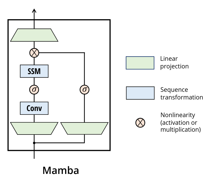
It resembles the structure of a GLU unit. We up-project, split into 2 path, left branch we convolve (depthwise convolution here), sigmoid, then run the SSM. Right branch we just sigmoid. Then we multiply them, and down-project back into embedding dimension.
Initializing the model
We create the Mamba block,
1
2
3
4
5
6
7
8
9
class MambaBlock(nn.Module):
    def __init__(self, embed_dim, inner_dim, state_dim, delta_rank):
        super().__init__()
        self.embed_dim = embed_dim
        self.inner_dim = inner_dim
        self.state_dim = state_dim
        self.delta_rank = delta_rank

        self.in_proj = nn.Linear(embed_dim, inner_dim * 2, bias=False)
The up-projection is done without biases, to form the left and right branch. Now we create convolution,
1
2
3
4
5
6
7
self.conv1d = nn.Conv1d(
    in_channels=inner_dim,
    out_channels=inner_dim,
    kernel_size=4,
    groups=inner_dim,
    padding=3,
)
You may find the kernel size and paddings a bit odd. However, this is normal, as it is a causal convolution. Try to visualize the first output of the convolution, it will consist of 3 pads and 1 token. Crucially, it does not contain future tokens. Basically prevents the model from cheating by looking at the next tokens using the convolution. Later on, we will only take the first L tokens of the convolution output, where L is the sequence length.
Now we want to form delta, B, and C. We will just make 1 linear layer, and split it later for efficiency.
1
2
self.x_proj = nn.Linear(inner_dim, delta_rank + state_dim * 2, bias=False)
self.dt_proj = nn.Linear(delta_rank, inner_dim, bias=True)
Note how delta is formed in 2 cycles. This is because we want to lower the rank of the delta matrix. Why? In the paper, under interpretation of delta, authors state,
Δ controls the balance between how much to focus or ignore the current input xt
Authors do not state this, but I suspect the lowering of rank allows for each token to be forced to decide how much to express itself in very few (say 1-2) scalars, which makes logical sense, as the vector of each token should be treated as a whole embedding, not piecewise.
We then initialize the weights such that delta stays between 0.1 and 0.001, as they do in S4,
1
2
3
4
5
6
7
8
9
10
11
12
13
14
# Initialize special dt projection to preserve variance at initialization
dt_init_std = self.delta_rank**-0.5
nn.init.uniform_(self.dt_proj.weight, -dt_init_std, dt_init_std)

# Initialize dt bias so that F.softplus(dt_bias) is between dt_min and dt_max
dt = torch.exp(
    torch.rand(inner_dim) * (math.log(0.1) - math.log(0.001))
    + math.log(0.001)
).clamp(min=1e-4)
# Inverse of softplus: https://github.com/pytorch/pytorch/issues/72759
inv_dt = dt + torch.log(-torch.expm1(-dt))
with torch.no_grad():
    self.dt_proj.bias.copy_(inv_dt)
self.dt_proj.bias._no_reinit = True
Now, we initialize the A matrix,
1
2
A = torch.arange(1, state_dim + 1).unsqueeze(0).repeat(inner_dim, 1)
self.A_log = nn.Parameter(torch.log(A))
We initialize it such that A looks something like this,
1
2
3
4
tensor([[1., 2., 3.],
        [1., 2., 3.],
        ...
        [1., 2., 3.]])
This is in accordance with the initialization used in S4D-real.
Finally, finish up with D and the down-projection,
1
2
self.D = nn.Parameter(torch.ones(inner_dim))
self.out_proj = nn.Linear(inner_dim, embed_dim, bias=False)
Great! We are finally done with initializations. Now, we will implement the logic.
Implementing architecture
Ok so first we will do up the basic architecture as shown earlier,
1
2
3
4
5
6
7
8
9
10
11
12
def forward(self, x):
    (b, l, d) = x.shape

    x_and_res = self.in_proj(x)  # shape (b, l, 2 * d_in)
    (x, res) = x_and_res.split(split_size=[self.inner_dim, self.inner_dim], dim=-1)
    x = x.transpose(-1, -2)
    x = self.conv1d(x)[:, :, :l]
    x = x.transpose(-1, -2)
    x = F.silu(x)
    y = self.ssm(x)
    y = y * F.silu(res)
    return self.out_proj(y)
This is basically a 1:1 copy of the architecture, is quite trivial. Now on to the hard part, the SSM.
Implementing SSM
We start off with taking the negative exponential of A,
1
2
3
(d_in, n) = self.A_log.shape
A = -torch.exp(self.A_log.float())
D = self.D.float()
We take exponential as we initialized it with a log, and negative as that is what is recommended by the S4D paper (it is due to something related to HiPPO theory I believe, but am not too sure).
Now we up-project x, and obtain B, C, and delta.
1
2
3
4
x_dbl = self.x_proj(x)  # (b, l, dt_rank + 2*n)
# delta: (b, l, dt_rank). B, C: (b, l, n)
(delta, B, C) = x_dbl.split(split_size=[self.delta_rank, n, n], dim=-1)
delta = F.softplus(self.dt_proj(delta))  # (b, l, d_in)
Finally, we run the scan of the SSM, this is basically the recurrent part of it,
1
return selective_scan(x, delta, A, B, C, D)
Now how do we implement this scan?
Implementing scan
This scan is to run the equation,
\[\displaylines{ x_{t} = \bar{A}x_{t-1} + \bar{B}u_{t}\\ y_{t} = Cx_{t} + Du }\]over all the u steps.
We create the dA tensor, by multiplying dt with A. We create a $\bar{A}$ and $\bar{B}$ tensor for each u step, and calculate the $\bar{B}u_{t}$. Then, we clamp dA for numerical stability.
1
2
3
4
def selective_scan(u, dt, A, B, C, D):
    dA = torch.einsum('bld,dn->bldn', dt, A)
    dB_u = torch.einsum('bld,bld,bln->bldn', dt, u, B)
    dA = dA.clamp(min=-20)
And as $\bar{A}$ is not constant over time, we need to solve for,
\[\begin{bmatrix} \bar{A}_{0}\\ \bar{A}_{1}\bar{A}_{0}\\ ...\\ \bar{A}_{t}\bar{A}_{t-1} ... \bar{A}_{0} \end{bmatrix}\]We do this like this,
1
2
padding = (0,  0,  0,  0,  1,  0)
dA_cumsum = F.pad(dA[:,  1:], padding).cumsum(1).exp()
We zero out the first embedding, then take a cumulative sum then exponential over this. By laws of exponents, this would result in the additions becoming multiplications effectively. This allows us to obtain the desired matrix!
Now the next few lines are the most confusing, so here is the code first, then I will explain,
1
2
x = dB_u / (dA_cumsum + 1e-12)
x = x.cumsum(1) * dA_cumsum
So after the first line,
\[x = [\frac{\bar{B}u_{0}}{\bar{A}_{0}}, \frac{\bar{B}u_{1}}{\bar{A}_{0}\bar{A}_{1}}, ..., \frac{\bar{B}u_{t}}{\bar{A}_{0}\bar{A}_{1}...\bar{A}_{t}}]\]Then we cumsum,
\[x = [\frac{\bar{B}u_{0}}{\bar{A}_{0}}, \frac{\bar{B}u_{0}}{\bar{A}_{0}} + \frac{\bar{B}u_{1}}{\bar{A}_{0}\bar{A}_{1}}, ..., \frac{\bar{B}u_{0}}{\bar{A}_{0}} +...+\frac{\bar{B}u_{t}}{\bar{A}_{0}\bar{A}_{1}...\bar{A}_{t}}]\]And remember, dA_cumsum has,
And when we multiply, x becomes,
\[x = [\bar{B}u_{0}, \bar{A}_{1}\bar{B}u_{0} + \bar{B}u_{1}, ..., (\bar{A}_{t}...\bar{A}_{1})\bar{B}u_{0} + ... + \bar{B}u_{t}]\]This is precisely what we would have gotten had we used a naive scan algorithm! Except that, cumsum is incredibly fast, as we can use the prefix sum algorithm, which is super parallelizable, and we can do this very fast on a GPU! This very parallelizability, is exactly why Mamba and related SSMs are so popular now, compared to older generation RNNs like LSTM and GRU. We get great training speeds.
The hard part is now over, finally, we solve for y, and return $Cx_{t} + Du$,
1
2
y = torch.einsum('bldn,bln->bld', x, C)
return y + u * D
And after all this work, we have finally implemented a Mamba block! Now, it is time to put it all together, and create a Mamba network!
Implementing Mamba network
For this, we will just do a classic transformer-like architecture. We will be doing sets of x = x + mamba(norm(x)). Then, we will take the final output of the model, and calculate loss for that. We will be doing this for Sequential MNIST classification, in which we feed the model a picture from MNIST in a stream.
1
2
3
4
5
6
7
8
9
10
11
12
13
14
15
16
17
18
19
20
21
22
23
24
25
class Model(nn.Module):
    def __init__(self, embed_dim, inner_dim, state_dim, n_layers):
        super().__init__()
        self.mambas = nn.ModuleList([])
        self.embeds = nn.Linear(1, embed_dim)
        self.outs = nn.Linear(embed_dim, 10)
        for i in range(n_layers):
            self.mambas.append(
                nn.Sequential(
                    nn.modules.normalization.RMSNorm(embed_dim),
                    MambaBlock(embed_dim, inner_dim, state_dim, 1)
                )
            )
        self.final_norm = nn.modules.normalization.RMSNorm(embed_dim)
    def forward(self, x):
        x = x.flatten(1).unsqueeze(-1)
        x = self.embeds(x)
        for mamba in self.mambas:
            x = x + mamba(x)
        x = x[:, -1, :]
        x = self.final_norm(x)
        x = self.outs(x)
        return x
# we will use a small model for demo
model = Model(embed_dim = 8, state_dim = 128, inner_dim = 32, n_layers = 4).cuda()
Sequential MNIST
We will train the model for sequential MNIST, we resize to 10x10 for easier training,
1
2
3
4
5
6
7
8
9
10
11

transform = transforms.Compose([
    transforms.ToTensor(),
    transforms.Resize((10,10)),
    transforms.Normalize((0.1307,), (0.3081,))
])
train_dataset = datasets.MNIST(root='./data', train=True, download=True, transform=transform)
test_dataset  = datasets.MNIST(root='./data', train=False, download=True, transform=transform)

train_loader  = torch.utils.data.DataLoader(dataset=train_dataset, batch_size=256, shuffle=True)
test_loader   = torch.utils.data.DataLoader(dataset=test_dataset, batch_size=1024, shuffle=False)
Start training the model on 3e-3 for Adam,
1
2
3
4
5
6
7
8
9
10
11
12
13
criterion = nn.CrossEntropyLoss()
optimizer = optim.Adam(model.parameters(), lr = 3e-3)
for i in range(10):
    for j, (inp, trg) in enumerate(train_loader):
        optimizer.zero_grad()
        outs = model(inp.cuda())
        loss = criterion(outs, trg.cuda())
        if j % 10 == 0:
            print("loss:", loss.item())
            acc = (outs.cpu().argmax(dim = -1) == trg).sum() / len(trg)
            print("acc:", acc.item())
        loss.backward()
        optimizer.step()
Finally, evaluate the model,
1
2
3
4
5
6
7
8
total = 0
correct = 0
with torch.no_grad():
    for _, (inp, trg) in enumerate(test_loader):
        outs = model(inp.cuda())
        correct += (outs.cpu().argmax(dim = -1) == trg).sum()
        total += len(trg)
print(correct / total)
And that’s it! Congratulations, if you followed along, you have now trained a Mamba model for the sequential MNIST task. I got a final test accuracy of 92.24%, but I did not really try too hard.
All code is available here. But it is mostly a refactored version of mamba-tiny, which you should also check out.
Appendix: cumsum scan vs naive scan
If you were wondering just how much of a speed boost the parallelizable cumsum scan gave over a naive scan, I wrote a code to test just that,
1
2
3
4
5
6
7
8
9
10
11
12
13
14
15
16
17
18
19
20
21
22
23
24
25
26
27
28
29
30
31
32
33
34
35
36
37
38
39
40
41
42
43
44
45
46
47
48
49
50
51
52
53
54
55
56
57
58
59
60
import torch
from torch.nn import functional as F
from einops import rearrange, repeat, einsum

def naive_selective_scan(u, delta, A, B, C, D):
    (b, l, d_in) = u.shape
    n = A.shape[1]
    padding =  (0, 0, 0, 0, 1, 0)
    dA = einsum(delta, A, 'b l d_in, d_in n -> b l d_in n')
    dA = dA.clamp(min=-20)
    dA = F.pad(dA[:, 1:], padding)
    deltaA = torch.exp(dA)
    deltaB_u = einsum(delta, B, u, 'b l d_in, b l n, b l d_in -> b l d_in n')

    x = torch.zeros((b, d_in, n), device=deltaA.device)
    ys = []
    for i in range(l):
        x = deltaA[:, i] * x + deltaB_u[:, i]
        y = einsum(x, C[:, i, :], 'b d_in n, b n -> b d_in')
        ys.append(y)
    y = torch.stack(ys, dim=1)  # shape (b, l, d_in)

    y = y + u * D

    return y

def selective_scan(u, dt, A, B, C, D):
    dA = torch.einsum('bld,dn->bldn', dt, A)
    dB_u = torch.einsum('bld,bld,bln->bldn', dt, u, B)
    dA = dA.clamp(min=-20)

    padding =  (0, 0, 0, 0, 1, 0)

    dA_cumsum = F.pad(dA[:, 1:], padding).cumsum(1).exp()
    x = dB_u / (dA_cumsum + 1e-15)
    x = x.cumsum(1) * dA_cumsum
    y = torch.einsum('bldn,bln->bld', x, C)

    return y + u * D


u = -1 + 2 * torch.rand(2, 10000, 32).cuda()
dt = torch.ones(2, 10000, 32).cuda()
A =  -torch.rand(32, 16).cuda()
B = torch.rand(2, 10000, 16).cuda()
C = torch.rand(2, 10000, 16).cuda()
D = torch.rand(32).cuda()

import time
naive_selective_scan(u, dt, A, B, C, D)
t0 = time.time()
for i in range(5):
    naive_selective_scan(u, dt, A, B, C, D)
print("naive:", time.time() - t0)

selective_scan(u, dt, A, B, C, D)
t0 = time.time()
for i in range(5):
    selective_scan(u, dt, A, B, C, D)
print("cumsum:", time.time() - t0)
Output:
1
2
naive: 6.160594701766968
cumsum: 0.00433659553527832
That’s over 1000x faster for the cumsum version! Note that the results may differ (from what I see it occurs between timestep 30-40 typically) between versions as the cumsum version does have an epsilon term for numerical stability, but that small number also causes butterfly effect down the road. In any case, this insane speedup, especially for long sequences, makes such small errors more than reasonable.
References
- https://github.com/PeaBrane/mamba-tiny - Mamba tiny, what I mainly used for this post
- https://github.com/johnma2006/mamba-minimal - Mamba minimal, mamba tiny without the fast scan
- https://github.com/state-spaces/mamba/ - the original Mamba implementation
- https://arxiv.org/pdf/2312.00752 - Mamba paper
- https://arxiv.org/pdf/2206.11893 - S4D paper
- https://arxiv.org/pdf/2111.00396 - S4 paper
- https://arxiv.org/pdf/2008.07669 - HiPPO paper
- https://arxiv.org/pdf/1609.09106 - Hypernetworks paper
- https://en.wikipedia.org/wiki/Prefix_sum - Prefix sum algorithm