Hello all, today I will cover flow matching. Flow matching is a (somewhat) novel technique to image generation, that seems to outperform all existing techniques. It is the backbone of many modern models like Stable Diffusion 3. So we will start off with the beloved Literature Review, and look through existing technique. Full code is available here
Literature Review
So in the existing pools of techniques, we have these:
VAE
GAN
VAE-GAN
Diffusion
Flow matching
Training
Decent speed, albeit a bit wasteful - oftentimes the encoder is thrown away
Painful. Model collapse happens reasonably often.
Model collapse quite unlikely, but again, you throw away encoder and discriminator usually.
Pretty decent speeds, but there are many ways to screw up due to high amounts of math
Very good, trains very fast, and simple to implement
Inference speed
Good - single pass
Good
Good
Poor - often needs many passes to generate decent quality
Mid - Faster than diffusion, slower than single pass models
Quality
Trash - images are often blurry
Good
Good, but blurrier than pure GAN
Very good
Very good
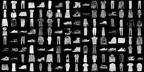
Overall, flow matching is a pretty good balance between speed, quality, and inference time. However, due to the high amounts of attention diffusion and flow matching models tend to use in the U-net, the models may require unwieldly amounts of VRAM and train time if we try to make the images any bigger than 128x128 or so. This is why latent diffusion (which can be trivially extended to flow matching) was invented, but we will not cover that today as we will just be working with the 28x28 Fashion MNIST dataset.
Math
I shall now cover the math of the flow matching techniques. I will casually ignore all the fancy probability and integrals used in the official paper (because admittedly I can’t understand a good chunk of it too), and use the simplest interpretation instead - the linear interpolation interpretation.
Let us start off by defining some terms. Let $x$ be the image, and $z$ be random noise. We start off at complete random noise at $t = 0$. Then all we need to do is draw a line (ie linearly interpolate) between $z$ and $x$, from $t = 0$ to $t = 1$. We will represent the model as $f$.
$$ x_{t} = xt + (1-t)z\\ \frac{dx_{t}}{dt} = x - z\\ f(x_{t}, t) = \frac{dx_{t}}{dt} = x - z $$
As such, all we have to do is train the model to find $x - z$, given $x_{t}$ and $t$.
Architecture
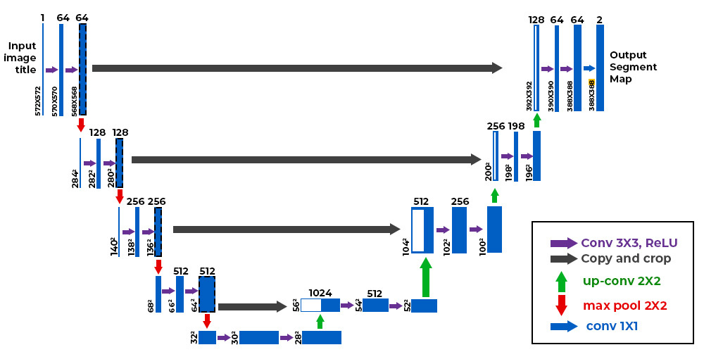
We will design the model in a classical U-net format, but after each of the convolution blocks, we introduce a self-attention. You can probably skip this whole section if you have implemented a diffusion model before.
Note this picture is just to give a rough idea of what a U-net looks like, we will implement something rather different
Time embedding
First we need to settle the time embedding, this we inject into every layer. Let $t$ be the time we want to obtain, $d$ be half the embedding dimension, and $x$ be the embedding.
$$ x_{i} = sin(\frac{t}{10000^{\frac{i}{d}}}) $$
We take this equation but cos instead of sin, and concat it, to form the entire embedding. Here it is in code:
defforward(self, x, t_emb): out = x resnet_input = out out = self.resnet_conv_first(out) out = out + self.t_emb_layers(t_emb)[:, :, None, None] out = self.resnet_conv_second(out) out = out + self.residual_input_conv(resnet_input) ifself.attend: batch_size, channels, h, w = out.shape in_attn = out.reshape(batch_size, channels, h * w) in_attn = self.attention_norms(in_attn) in_attn = in_attn.transpose(1, 2) out_attn, _ = self.attentions(in_attn, in_attn, in_attn) out_attn = out_attn.transpose(1, 2).reshape(batch_size, channels, h, w) out = out + out_attn out = self.down_sample_conv(out) return out
Note how we inject the time embedding in between the conv layers. We do this for every layer later as well. Another key thing to note is only downsample AFTER you do everything. And do the reverse for the upsampling portion later in the up block. Otherwise you’ll just get a total mess of an output. Not too sure how related, but do check out this article.
Middle block
I will skip the initialization code, it’s just the same as that of the downsampler. For this block, instead of resnet -> attention, we do resnet -> attention -> resnet.
defforward(self, x, t_emb): out = x resnet_input = out out = self.resnet_convs[0](out) out = out + self.t_emb_layers[0](t_emb)[:, :, None, None] out = self.resnet_convs[1](out) out = out + self.residual_input_conv[0](resnet_input)
batch_size, channels, h, w = out.shape in_attn = out.reshape(batch_size, channels, h * w) in_attn = self.attention_norms(in_attn) in_attn = in_attn.transpose(1, 2) out_attn, _ = self.attentions(in_attn, in_attn, in_attn) out_attn = out_attn.transpose(1, 2).reshape(batch_size, channels, h, w) out = out + out_attn resnet_input = out out = self.resnet_convs[2](out) out = out + self.t_emb_layers[1](t_emb)[:, :, None, None] out = self.resnet_convs[3](out) out = out + self.residual_input_conv[1](resnet_input) return out
classUpBlock(nn.Module): def__init__(self, in_channels, out_channels, t_emb_dim, up_sample=True, num_heads=4, attend = True): super().__init__() ... self.up_sample_conv = nn.ConvTranspose2d(in_channels // 2, in_channels // 2, 4, 2, 1) \ ifself.up_sample else nn.Identity() defforward(self, x, out_down, t_emb): x = self.up_sample_conv(x) x = torch.cat([x, out_down], dim=1) out = x resnet_input = out out = self.resnet_conv_first(out) out = out + self.t_emb_layers(t_emb)[:, :, None, None] out = self.resnet_conv_second(out) out = out + self.residual_input_conv(resnet_input) ifself.attend: batch_size, channels, h, w = out.shape in_attn = out.reshape(batch_size, channels, h * w) in_attn = self.attention_norms(in_attn) in_attn = in_attn.transpose(1, 2) out_attn, _ = self.attentions(in_attn, in_attn, in_attn) out_attn = out_attn.transpose(1, 2).reshape(batch_size, channels, h, w) out = out + out_attn return out
As you will note, we first upsample with ConvTranspose2d, then we concat with the respective downsample block, for the U-net residuals. We do this in the channel dimensions.
model.train() for epoch_idx inrange(num_epochs): losses = [] for im, _ in tqdm(train_dataloader): optimizer.zero_grad() im = im.float().to(device) im = (2 * im) - 1 t = torch.rand((im.shape[0])).to(device) noise = torch.randn_like(im).to(device) noisy_im = im * t[:, None, None, None] + (1 - t)[:, None, None, None] * noise v_pred = model(noisy_im, t)
loss = criterion(v_pred, im - noise) losses.append(loss.item()) loss.backward() optimizer.step() print('Finished epoch:{} | Loss : {:.4f}'.format( epoch_idx + 1, np.mean(losses), ))
Note how as mentioned, we are training the model to find $x - z$, given $x_{t}$ and $t$.
As for inference, we will just use simple Euler methods to solve the ODE represented with $\frac{dx_{t}}{dt}$, to find $x$ given completely random noise.
1 2 3 4 5 6 7 8 9 10 11 12 13 14 15
n_step = 100 model.eval() xt = torch.randn((128, 1, 28, 28)).to(device) with torch.no_grad(): for i in tqdm(range(n_step)): velo = model(xt, torch.as_tensor(i / n_step).unsqueeze(0).to(device)) xt = xt + velo / n_step